Easy Way to Calculate Gradient Descent on a Linear Regression Equation

Introduction linear regression with gradient descent

This tutorial is a rough introduction into using gradient descent algorithms to estimate parameters (slope and intercept) for standard linear regressions, as an alternative to ordinary least squares (OLS) regression with a maximum likelihood estimator. To begin, I simulate data to perform a standard OLS regression with maximum likelihood using sums of squares. Once explained, I then demonstrate how to substitute gradient descent simply and interpret results.

          library(tidyverse)  ## -- Attaching packages --------------------------------------- tidyverse 1.3.1 --  ## v ggplot2 3.3.5     v purrr   0.3.4 ## v tibble  3.1.3     v dplyr   1.0.7 ## v tidyr   1.1.3     v stringr 1.4.0 ## v readr   2.0.1     v forcats 0.5.1  ## Warning: package 'readr' was built under R version 4.1.1  ## -- Conflicts ------------------------------------------ tidyverse_conflicts() -- ## x dplyr::filter() masks stats::filter() ## x dplyr::lag()    masks stats::lag()                  

Ordinary Least Square Regression

Simulate data

Generate random data in which y is a noisy function of x

          set.seed(123)  x <- runif(1000, -5, 5) y <- x + rnorm(1000) + 3                  

Fit a linear model

          lm <- lm( y ~ x ) # Ordinary Least Squares regression with General Linear Model  mod <- print(lm)  ##  ## Call: ## lm(formula = y ~ x) ##  ## Coefficients: ## (Intercept)            x   ##      3.0118       0.9942  mod  ##  ## Call: ## lm(formula = y ~ x) ##  ## Coefficients: ## (Intercept)            x   ##      3.0118       0.9942                  

Plot the data and the model

          plot(x,y, col = "grey80", main='Regression using lm()', xlim = c(-2, 5), ylim = c(0,10));  text(0, 8, paste("Intercept = ", round(mod$coefficients[1], 2), sep = "")); text(4, 2, paste("Slope = ", round(mod$coefficients[2], 2), sep = "")); abline(v = 0, col = "grey80"); # line for y-intercept abline(h = mod$coefficients[1], col = "grey80") # plot horizontal line at intercept value abline(a = mod$coefficients[1], b = mod$coefficients[2], col='blue', lwd=2) # use slope and intercept to plot best fit line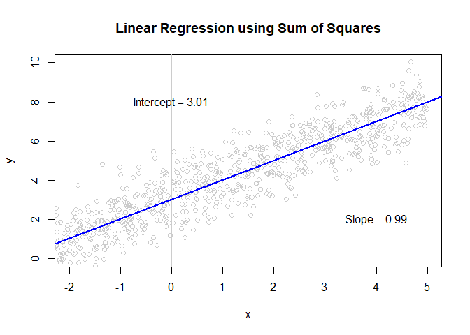                  

Calculate intercept and slope using sum of squares

          x_bar <- mean(x) # calculate mean of independent variable y_bar <- mean(y) # calculate mean of dependent variable  slope <- sum((x - x_bar)*(y - y_bar))/sum((x - x_bar)^2) # calculate sum of differences between x & y, and divide by sum of squares of x slope  ## [1] 0.9941662  intercept <- y_bar - (slope * x_bar) # calculate difference of y_bar across the linear predictor intercept  ## [1] 3.011774                  

Plot data using manually calculated parameters

          plot(x,y, col = "grey80", main='Regression with manual calculations', xlim = c(-2, 5), ylim = c(0,10));  abline(a = intercept, b = slope, col='blue', lwd=2)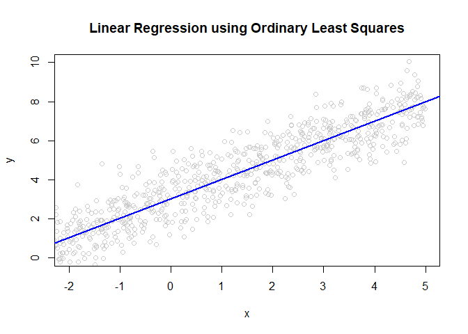                  

Gradient Descent:

Using the same simulated data as before, we will estimate parameters using a machine learning algorithm

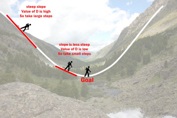
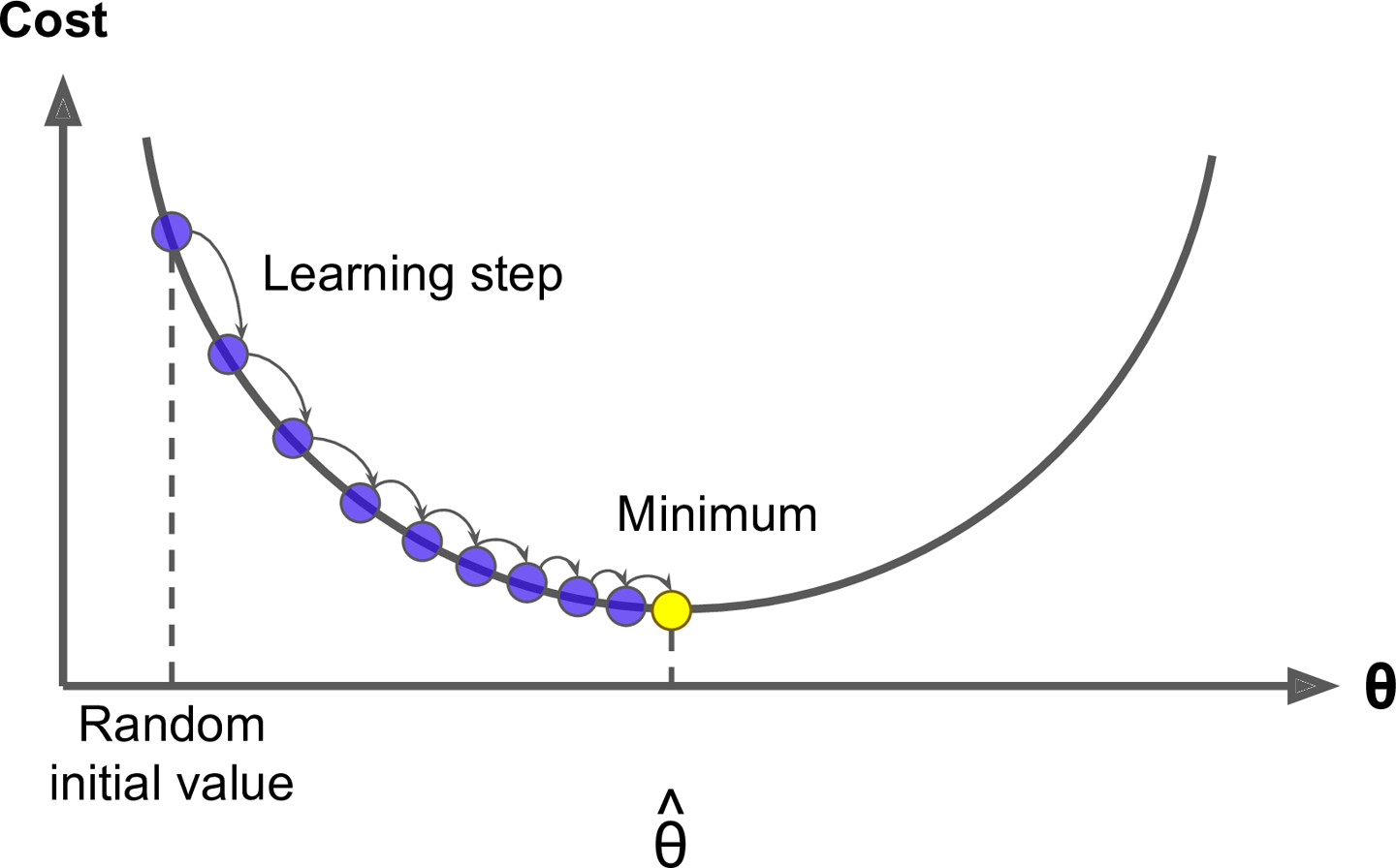
Here's some figures I found helpful while trying to understand how gradient descent works:

To determine the goodness of fit for a given set of parameters, we will empliment a Squared error cost function (a way to calculate the degree of error for a guess for slope and intercept)

          cost <- function(X, y, theta) {   sum( (X %*% theta - y)^2 ) / (2*length(y)) }                  

We must also set two additional parameters: learning rate and iteration limit

          alpha <- 0.01 num_iters <- 1000  # keep history cost_history <- double(num_iters) theta_history <- list(num_iters)  # initialize coefficients theta <- matrix(c(0,0), nrow=2)  # add a column of 1's for the intercept coefficient X <- cbind(1, matrix(x))  # gradient descent for (i in 1:num_iters) {   error <- (X %*% theta - y)   delta <- t(X) %*% error / length(y)   theta <- theta - alpha * delta   cost_history[i] <- cost(X, y, theta)   theta_history[[i]] <- theta }  print(theta)  ##           [,1] ## [1,] 3.0116439 ## [2,] 0.9941657                  

Plot data and converging fit

          iters <- c((1:31)^2, 1000) cols <- rev(terrain.colors(num_iters)) library(gifski) png("frame%03d.png") par(ask = FALSE)  for (i in iters) {   plot(x,y, col="grey80", main='Linear regression using Gradient Descent')   text(x = -3, y = 10, paste("slope = ", round(theta_history[[i]][2], 3), sep = " "), adj = 0)   text(x = -3, y = 8, paste("intercept = ", round(theta_history[[i]][1], 3), sep = " "), adj = 0)   abline(coef=theta_history[[i]], col=cols[i], lwd = 2) }  dev.off()  ## png  ##   2  png_files <- sprintf("frame%03d.png", 1:32) gif_file <- gifski(png_files, delay = 0.1) unlink(png_files) utils::browseURL(gif_file)                  

Calculate intercept and slope using gradient descent (Machine Learning):

          plot(cost_history, type='line', col='blue', lwd=2, main='Cost function', ylab='cost', xlab='Iterations')  ## Warning in plot.xy(xy, type, ...): plot type 'line' will be truncated to first ## character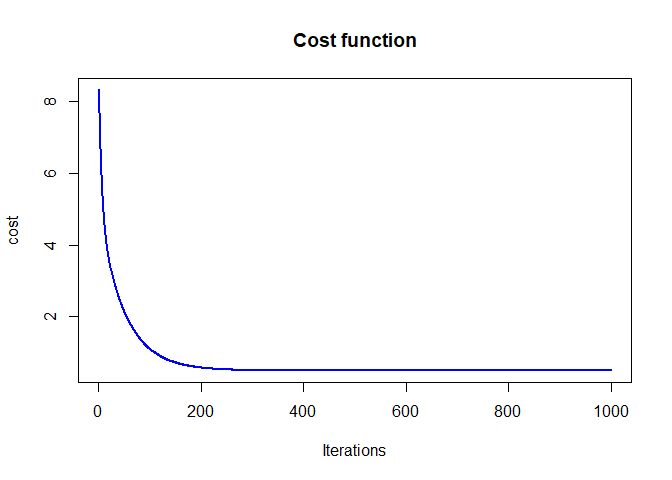                  

Using gradient descent with real data

I'll demonstrate it's features using an existing dataset from Bruno Oliveria: "Amphibio":
• Link to publication: https://www.nature.com/articles/sdata2017123
• Link to data: https://ndownloader.figstatic.com/files/8828578

Load amphibio data!

          install.packages("downloader") library(downloader)  url <- "https://ndownloader.figstatic.com/files/8828578" download(url, dest="lrgb/amphibio.zip", mode="wb")  unzip("lrgb/amphibio.zip", exdir = "./lrgb")  df <- read_csv("AmphiBIO_v1.csv") %>%   select("Order",          "Body_mass_g",          "Body_size_mm",          "Size_at_maturity_min_mm",          "Size_at_maturity_max_mm",          "Litter_size_min_n",          "Litter_size_max_n",          "Reproductive_output_y") %>%   na.omit %>%   mutate_if(is.numeric, ~ log(.))  ## Rows: 6776 Columns: 38  ## -- Column specification -------------------------------------------------------- ## Delimiter: "," ## chr  (6): id, Order, Family, Genus, Species, OBS ## dbl (31): Fos, Ter, Aqu, Arb, Leaves, Flowers, Seeds, Arthro, Vert, Diu, Noc... ## lgl  (1): Fruits  ##  ## i Use `spec()` to retrieve the full column specification for this data. ## i Specify the column types or set `show_col_types = FALSE` to quiet this message.  plot(df$Body_size_mm, df$Size_at_maturity_max_mm, col = "grey80", main='Correlation of amphibian traits', xlab = "Body size (mm)", ylab = "Max size at maturity (mm)");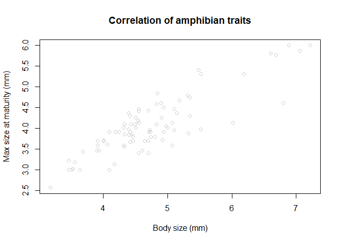                  

Fit a linear model

          lm <- lm(Size_at_maturity_max_mm ~ Body_size_mm, data = df) # Ordinary Least Squares regression with General Linear Model  mod <- print(lm)  ##  ## Call: ## lm(formula = Size_at_maturity_max_mm ~ Body_size_mm, data = df) ##  ## Coefficients: ##  (Intercept)  Body_size_mm   ##       0.6237        0.7265  mod  ##  ## Call: ## lm(formula = Size_at_maturity_max_mm ~ Body_size_mm, data = df) ##  ## Coefficients: ##  (Intercept)  Body_size_mm   ##       0.6237        0.7265                  

Plot the data and the model

          plot(df$Body_size_mm, df$Size_at_maturity_max_mm, col = "grey80", main='Linear Regression using Sum of Squares', xlab = "Body size (mm)", ylab = "Max size at maturity (mm)");  text(4, 5, paste("Intercept = ", round(mod$coefficients[1], 2), sep = "")); text(6, 3, paste("Slope = ", round(mod$coefficients[2], 2), sep = "")); abline(a = mod$coefficients[1], b = mod$coefficients[2], col='blue', lwd=2) # use slope and intercept to plot best fit line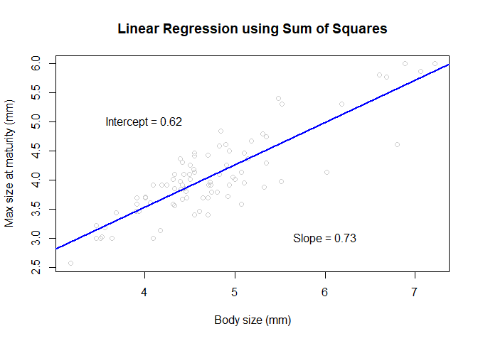                  

Calculate intercept and slope using sum of squares

          x <- df$Body_size_mm y <- df$Size_at_maturity_max_mm x_bar <- mean(x) # calculate mean of independent variable y_bar <- mean(y) # calculate mean of dependent variable  slope <- sum((x - x_bar)*(y - y_bar))/sum((x - x_bar)^2) # calculate sum of differences between x & y, and divide by sum of squares of x slope  ## [1] 0.7264703  intercept <- y_bar - (slope * x_bar) # calculate difference of y_bar across the linear predictor intercept  ## [1] 0.6237047  ### plot data using manually calculated parameters plot(x,y, col = "grey80", main='Linear Regression using Ordinary Least Squares', xlab = "Body size (mm)", ylab = "Max size at maturity (mm)");  abline(a = intercept, b = slope, col='blue', lwd=2)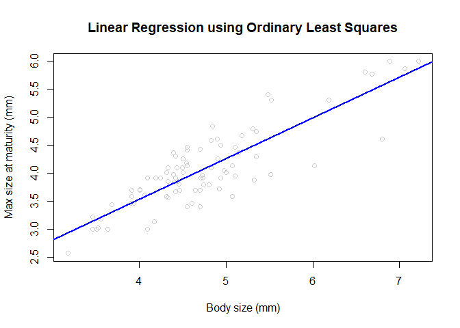                  

Calculate intercept and slope using gradient descent (Machine Learning)

Squared error cost function (a way to calculate the degree of error for a guess for slope and intercept)

          ### learning rate and iteration limit alpha <- 0.001 num_iters <- 1000  ### keep history cost_history <- double(num_iters) theta_history <- list(num_iters)  ### initialize coefficients theta <- matrix(c(0,0), nrow=2)  ### add a column of 1's for the intercept coefficient X <- cbind(1, matrix(x))  # gradient descent for (i in 1:num_iters) {   error <- (X %*% theta - y)   delta <- t(X) %*% error / length(y)   theta <- theta - alpha * delta   cost_history[i] <- cost(X, y, theta)   theta_history[[i]] <- theta }  print(theta)  ##           [,1] ## [1,] 0.1816407 ## [2,] 0.8175962                  

Plot data and converging fit

          plot(x,y, col="grey80", main='Linear regression using Gradient Descent', xlab = "Body size (mm)", ylab = "Max size at maturity (mm)") for (i in c((1:31)^2, 1000)) {   abline(coef=theta_history[[i]], col="red") } abline(coef=theta, col="blue", lwd = 2)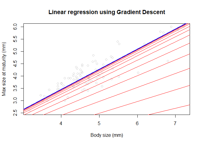                  

          plot(cost_history, type='line', col='blue', lwd=2, main='Cost function', ylab='cost', xlab='Iterations')  ## Warning in plot.xy(xy, type, ...): plot type 'line' will be truncated to first ## character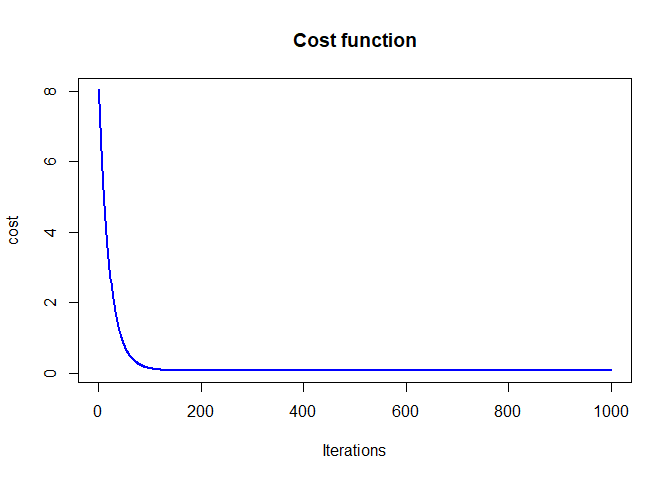                  

castillovizienteling.blogspot.com

Source: https://www.alexbaecher.com/post/gradient-descent/

Share this post